Written by John Kesler

Retrospect (edit: Feb 2021)

Yeah, this was _insanely_ optimistic at best, in retrospect. I think that the bulk of the content here is solid in terms of discussing simple models and basic fitness functions and all that, but don't take the predictions or anything here too seriously ;). After all, it was hurriedly made as a capstone project, and I *absolutely* do not have a background in any of the stuff being discussed here except the math

There's probably something interesting to be said about the potential damage of a bunch of non-experts suddenly swarming a topic and contributing what they know to it... Clearly there are good side effects (people become deeply interested, more lower level things are made to hook people), but also there are some undeniable downsides. Dunning-Kruger effect much lol?

The Usage of Epidemiological Models

Ever since scientists and researchers have acknowledged the presence of diseases, people have been interested in finding ways of modeling and predicting their spread. Many of the tools used to make those predictions -- epidemiological models -- have recently been under the limelight due to the current outbreak of COVID-19, so I've been interested in looking at and learning more about how they work.

In the past decade, the tools and techniques used when constructing and evaluating epidemiological models have become both, more powerful, as well as more accessible to the general public thanks to advances in computer science. These advances have led to a novel blend of machine learning and epidemiological techniques that can be applied when developing models to track the spread of diseases.

Throughout the past couple of weeks, I've looked into some of the ways to apply machine learning techniques to a couple of types of epidemiological models, in search of new ways to look at and understand how the Coronavirus has spread in the past, and hopefully understand how it might continue to spread in the following weeks.

Modelling Exponential Growth

One of the most commonly used epidemiological models is a simple exponential model that makes use of the basic reproductive number of a disease, or \(R_0\) (pronounced R-naught). Functionally, the \(R_0\) value is the number of people that we expect each infected person to continue to infect, so if it's between 2-3 for a disease, we expect that a person who becomes infected will infect 2-3 people while they remain contagious. For a disease like the common cold, it usually falls around 2, while a faster spreading disease such as smallpox (which has an \(R_0\) value of about 5) is much higher.

If we know how many people one person is likely to infect, then we should be able to form predictions of how many people will be infected in the future -- it's basically exponential growth, where the rate of growth is controlled by the \(R_0\) value. One of the advantages of using such a simple model is that it's incredibly easy to build, or "fit", the model to align with and predict the spread of diseases. Basic exponential models when used to model the spread of diseases are generally expressed like so (where \(N(t)\) is the number of people infected at a certain time, \(t\), after the first infection, and \(\tau\) is how long someone is infected):

After running a fit of this model on the worldwide COVID-19 data while the number of infected cases was still rising exponentially (so, only including about the first month and a half of data), the exponential model found that COVID-19's \(R_0\) value was roughly 1.2, (with an \(R^2\) of .92 for the fit). More accurate models built using similar data (and not using a simple exponential model) estimate that the \(R_0\) value of COVID-19 is actually between 3.8 and 8.9.

Strengths and Weaknesses of the Exponential Model

As you can probably tell from the disparity in the results of my basic exponential model compared to a more accurate one, the exponential model must be flawed -- and it is. The model itself has a minimal use case: outside of the period where the disease initially spreads without interference, an exponential model will fail. It's reasonably easy to notice why it might not perform well, as eventually the spread of the disease will either be artificially slowed down by people flattening the curve and lowering the effective \(R_0\) value, or because of the virus naturally spreading so much that it reaches the carrying capacity of the population, at which point it can't spread anymore.

Even though an exponential model is clearly not accurate enough to make predictions, the \(R_0\) value obtained can still be useful -- also, there are alternative ways of finding it that take advantage of features present in another, more accurate, kind of model known as a compartmental model. Thanks to the \(R_0\) value having a real-world meaning and being relatively constant when a disease initially spreads, it's at least useful when looking at the initial spread of diseases and comparing them to each other.

Compartmental Models

An alternative, and much more commonly used, epidemiological model is the compartmental model. This type of model is reasonably easy to understand -- when considering the spread of a disease, there are a few "compartments" or categories that people will fall under. Either a person hasn't been infected yet, so they're Susceptible, they've been Infected and are currently capable of spreading the disease, or they've Recovered from the disease and are both immune to it and no longer contagious (note that fatalities are considered recovered when using this model). One of the most basic compartmental models, a SIR model, models the spread of disease by moving people between those three compartments based on how many people are in other compartments.

Mathematically, the SIR model is easy to conceptually understand, as there are only a couple of parameters that determine how the model behaves. The rate of infection (represented by \(\beta\)) is the rate at which susceptible people become infected, and the recovery constant (\(\gamma\)) is the rate at which infected people recover.

One of the challenges with using a SIR model is that it generally has to be solved iteratively, meaning that in order to predict how many people are infected at a given point in the future, you have to first calculate how many people are infected at every time before that point. This is because the rate at which people move between compartments at a given time is defined by how many people are in each compartment. The upside to this, however, is that the model can be represented with only three formulas that define the change in each category's population:

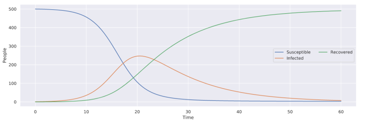
Using only those three equations, it's reasonably easy to model the spread of an arbitrary disease with a given \(\beta\) and \(\gamma\) value -- in this case, \(\beta = .001\) and \(\gamma = .1\).

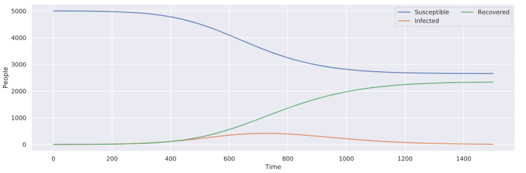
Even though the SIR model accounts for how many people are infected as well as how many people can be affected, which fixes one of the critical issues with the exponential model, it still makes an assumption that the intrinsic values defining the spread of the disease remain constant. To me, this assumption doesn't make sense at face value, as it's also reasonable to assume that people will take actions against the spread of the disease, which will change the rate of infection (\(\beta\)). When developing my model, I decided to handle this problem by not making \(\beta\) constant, but instead defined as a function of time, meaning that it can change as time progresses. Through the use of this change, the point at which a disease is no longer modeled to spread (i.e., no more new cases) is no longer restricted to the point where there are no more susceptible people, but rather to when the disease is no longer infectious (\(\beta=0\)). With my model below (of an arbitrary disease), note that there are people that remain susceptible after the disease stops spreading, unlike with the basic SIR model above.

Fitting Models

When creating any kind of forecast, there are generally two main tasks that need to be accomplished -- first, a representation of the process being modeled needs to be created that takes in parameters (in the case of the SIR model, \(\beta\) and \(\gamma\)) and produces a result, and secondly, the parameters must be changed so that the model accurately reflects the process being represented. To deal with the second task, one must "fit" their model by changing the parameters and seeing how the model performs when compared to real-world data.

The key to understanding how models are fit is that any possible combination of parameters will create a different model, which, when being tested against a set of constant, real-world data, will give us a specific "error" (how badly it performs, lower is good). Keeping that in mind, we can create a new function, which takes in a set of parameters as an input and gives us an error as an output -- this new function is what's known as a "loss function", and our goal is to figure out what inputs we need to provide to minimize the output.

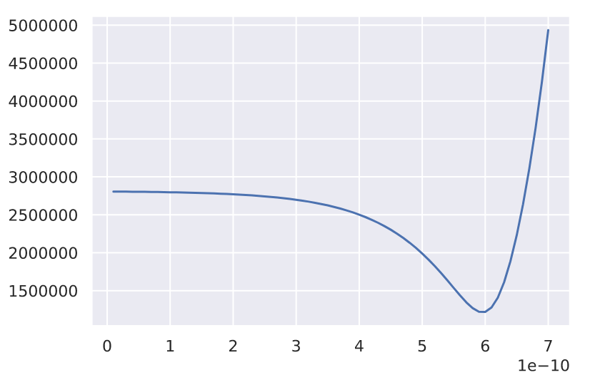A basic loss function, error on the y-axis, potential values for a parameter on the x-axis

The graph above is an example of what a loss function might look like, with a parameter that we can change on the x-axis and the corresponding error on the y-axis. It's pretty easy to see where the lowest point is and what the best parameter that we can choose to minimize the error is -- unfortunately the challenge of minimizing the error becomes exponentially more difficult as we increase the number of parameters, as the volume of the space that we are looking at exponentially increases. You can pretty easily tell where the lowest error is with only one parameter, but what if there are two parameters, or even three, like in the SIR model that I developed before (where \(\beta\) is a function of time: \(\beta(t) = at+b\)).

A sampled cost function with a boat about to perform gradient descent

How should one optimize a model with infinitely many parameters? Unfortunately, there isn't a general solution to model optimization, as often a model can't be stated as a differentiable function (which would let us find the points where it levels off or use a slope field to our advantage), and every model will perform differently from each other. Nevertheless, there are still many powerful techniques that we can take advantage of, especially if our model's loss function looks a certain way. When optimizing basic SIR models, I found that their loss functions will generally look like a smooth hill or waterfall, which lets us take advantage of an optimization technique called gradient descent.

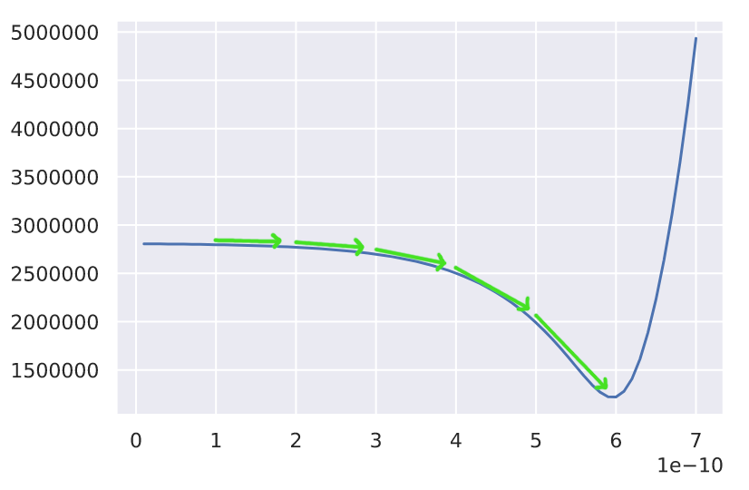An example of gradient descent with a constant step size.

In the case where a graph of the loss function is smooth (and not bumpy, which introduces multiple minima), we can simply optimize the model by taking steps in the downwards direction until we reach the bottom of the graph or the minimum error. The implementation of gradient descent that I ended up using involves a few steps to optimize a SIR model's parameters:

1. First, pick a set of random parameters that make sense (as in aren't impossible, for a SIR model this generally involves restricting the \(\beta\) and \(\gamma\) values to be small numbers)
2. Make adjustments to the parameters based on the current learning rate in all the possible directions that the error can move along our cost function's parameter axes
3. Pick the set of adjusted parameters that takes us to the new lowest error
4. Repeat from step 2 for a number of "epochs" (how many steps we take)

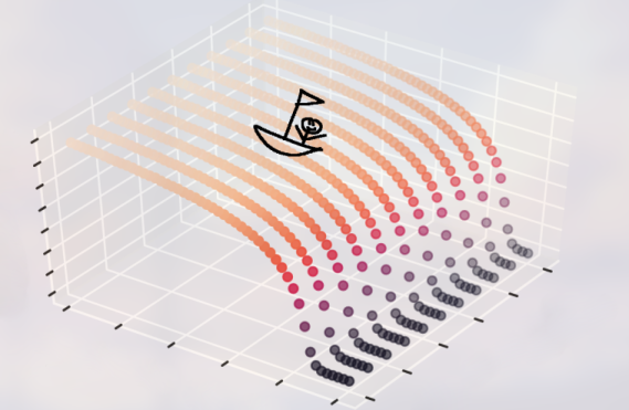
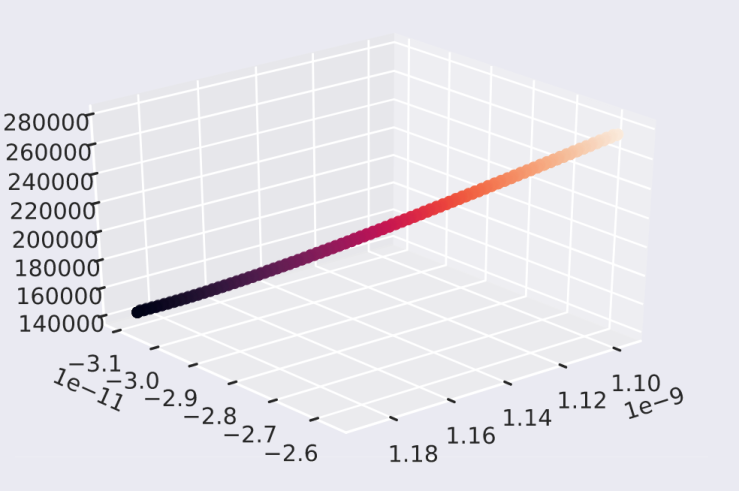This is a visualization of one of the actual paths that my model ended up taking to be optimized -- as you can see, it goes from relatively high error (on the y-axis/color) to what appears to be a minimum while taking a very smooth path

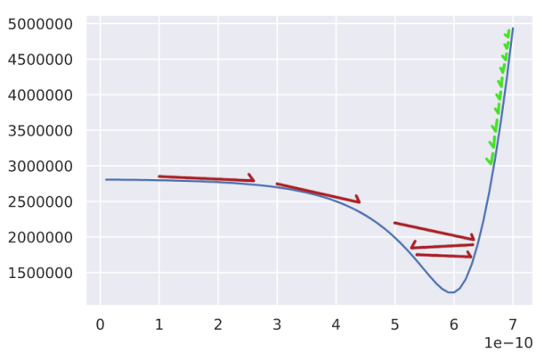
Most of the challenges with optimizing models come in at this point, where we have to go about optimizing the hyperparameters of the optimizer (the things that control how the optimization behaves). For example, we need to determine the size of the steps that the model takes as it's being optimized -- this is what's known as the "learning rate". A learning rate that is too large will lead to issues like with what the red steps are doing in the above graph; we'll often step over the minimum error, and continue oscillating back and forth without making any progress. Learning rates that are too small (in green) are often less problematic as the optimization process will almost always make it to the minima, but it will often take a large number of epochs to do that, which makes us wait an unreasonable amount of time for the model to be fit.

Challenges with SIR Models

Unfortunately, even though the SIR model is a much more versatile and potentially more accurate model (as compared to an exponential model), there are many model-specific challenges that arise when fitting them to follow the spread of diseases. The first, and most prominent one, is due to the additional parameter brought in when using a non-constant \(\beta\) value -- without realizing it, making \(\beta\) non-constant led to the loss function no longer being smooth, giving us many minimum errors that the model could arrive in. Even though more parameters will almost always lead to more flexibility, and in turn, less training error, it also means that there's more complexity involved when fitting the model.

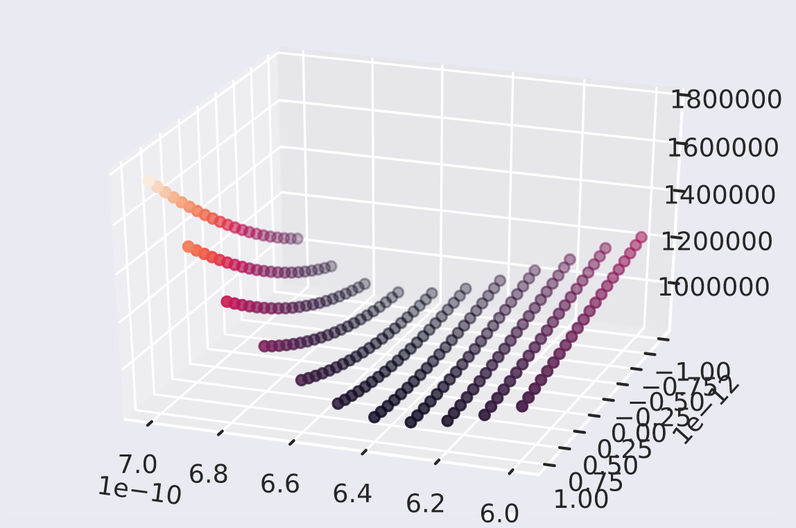The x and z-axes are the parameters, in this case, \(\beta\) and \(\gamma\)

This issue persisted even when going back to a model with a constant \(\beta\) value, as instead of having a single point/hole which the model could arrive in, there were multiple in the form of a valley. The presence of a valley implies that there are many different solutions that will perform equivalently well within the data that we currently have -- this leads us to the other major issue with the SIR model, in that there are multiple combinations of parameters which will give us similar-looking results, but only for a small slice of time. Outside of that initial slice of time that the SIR model trains in, it can deviate in many different ways, and without knowing more about the spread of a disease, such as when cases peak, it's difficult to make a confident guess using the discussed optimization methods (that is to say, we can't extrapolate data using a SIR model).

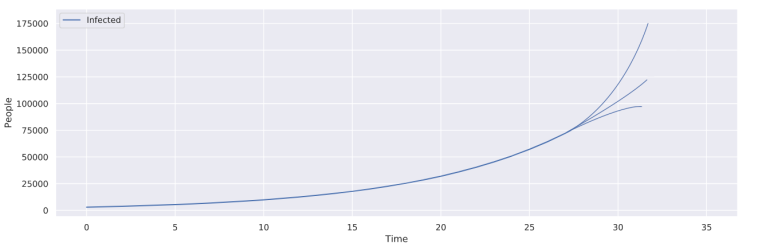Potential ways in which a SIR model might deviate, all of which are possible given the non-constant \(\beta\) value

Final Thoughts

Ultimately, until we know the overall trend of how the current outbreak of COVID-19 will propagate, it's unlikely that either the SIR model or the exponential model that I developed will converge and become accurate. This, in turn, means that they won't be useful for developing predictions about the future, or drawing overall conclusions about the spread of the disease as I originally intended. There are still some important takeaways about the use cases of each model and how they might be able to be improved in the future.

Simple exponential models, while definitely not accurate outside of the initial growth period that diseases go through, can still be used as a basic way of finding the \(R_0\) value of a pandemic, in turn letting us compare it to other outbreaks. SIR models are an effective way of modeling the spread of a disease once it has happened, but without using some other kind of model to aid in narrowing down the potential trajectories that a disease might take, it will be hard, if not impossible, to make predictions about the spread of diseases.

Overall, without having more data, it's hard to make accurate predictions about the progression of COVID-19 using the techniques that I discussed, but once that data is in place, the models should function reasonably well, allowing for us to draw conclusions about how COVID-19 has spread.